This image shows the inertial pendulum with mass added to the end. The blue strip of tape passes through a photogate which measures the period of oscillation of the inertial pendulum. Each period corresponds to the specific mass added to the pendulum.
Starting the process of creating the "lnT = nln(m +Mtray) + lnA" graph began with collecting data. The image above shows the resulting period, T, of various masses added to the inertial pendulum. This data was developed into a graph that would eventually be altered to display "lnT" on the y-axis and "ln(m + Mtray)" on the x-axis.
This graph, and the following graphs as well, represent the model "lnT = nln(m + Mtray) + lnA". These graphs allow us to derive "n", the slope th of graph, and "A" the y-intercept of the graph as well. However, in order to obtain a straight line, we had to guess the mass of the tray, Mtray. In this case, a mass of 280g was assigned to be the mass of the tray. Doing this resulted in a correlation of 0.9995, which is a good indicator that our line is straight.
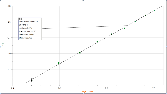
This graph produced the highest correlation, 0.9996. The mass assigned to the tray was 300g.
Lastly, this graph produced the lowest correlation, 0.9994. The mass assigned to the tray was 340g. At this point, each graph yields information that we can use in the model "T = A|(m + Mtray)^n"; these graphs provide us with "n", "A", and Mtray.
Now that we can apply these variables (with known values) into the aforementioned model, it was our job to place the objects with unknown masses (an eraser and a wallet) on the tray of the inertial pendulum and discover what their period of oscillation was. While we actually weighed the objects to know what their masses are, the purpose of finding the period of their oscillations was so that we could use it in the model "T = A(m + Mtray)^n". We now have what we did not have at the start of the lab; we have four known variables and one unknown variable. Solving for "m", the mass added to the tray, becomes a question of math.
Using the information we derived from the "lnT" models and period of oscillation for each unknown mass, we were able to solve the "T" model for "m" and compare the calculated mass to the actual mass of the unknown objects.The values for Mtray, "n", and "A" were applied to each unknown mass and its corresponding period. The result: six measurements for the calculated mass of the unknown masses (which we knew). The calculated mass for each were close to the actual mass of the objects for each time we solved the equations.
Although we tried our best to be as precise as possible and follow the directions as best as we could, there were some things that we could have done better. For one, we were not sure exactly where to place the masses/objects on the tray of the inertial pendulum. The masses/objects swayed side-to-side as the inertial pendulum moved.


Probably a closer approximation of the purpose was to develop a mathematical model of how the inertial pendulum works, and then check out the model by using it to find the mass of an "unknown" object.
ReplyDeleteThe y-intercept is ln(A).
The approach to finding Mtray was to find the range of masses that give the highest possible correlation rather than nearly the highest possible correlation.
Somewhere near the beginning you might say something about developing the model by measuring the period for a variety of masses added to the inertial pendulum.
Probably your period data should have more significant figures to it. The photogate usually gives four or five digits.
Your calculations are fine. The lab handout had a suggested format for reporting your results.
As far as uncertainties go . . . When we set up our original equation all of the masses were cylinders centered in the tray.
Our unknown objects had different shapes and perhaps different placement in the tray. We didn't test separately to see if placement or shape made a difference. This isn't a human error so much as an assumption (that mass is the only variable) that maybe turns out not to be true.